Create and track plots from experiments
3 minute read
wandb.plot のメソッドを使用すると、トレーニング中に時間とともに変化するグラフを含め、wandb.log でグラフを追跡できます。カスタムグラフ作成フレームワークの詳細については、このガイドを確認してください。
基本的なグラフ
これらのシンプルなグラフを使用すると、メトリクスと結果の基本的な可視化を簡単に構築できます。
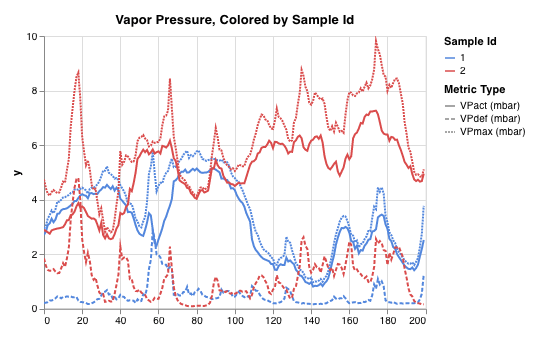
wandb.plot.line()
カスタム折れ線グラフ (任意の軸上の接続された順序付きポイントのリスト) を記録します。
data = [[x, y] for (x, y) in zip(x_values, y_values)]
table = wandb.Table(data=data, columns=["x", "y"])
wandb.log(
    {
        "my_custom_plot_id": wandb.plot.line(
            table, "x", "y", title="Custom Y vs X Line Plot"
        )
    }
)
これを使用して、任意の2つの次元で曲線を記録できます。2つの値のリストを互いにプロットする場合、リスト内の値の数は正確に一致する必要があります。たとえば、各ポイントにはxとyが必要です。
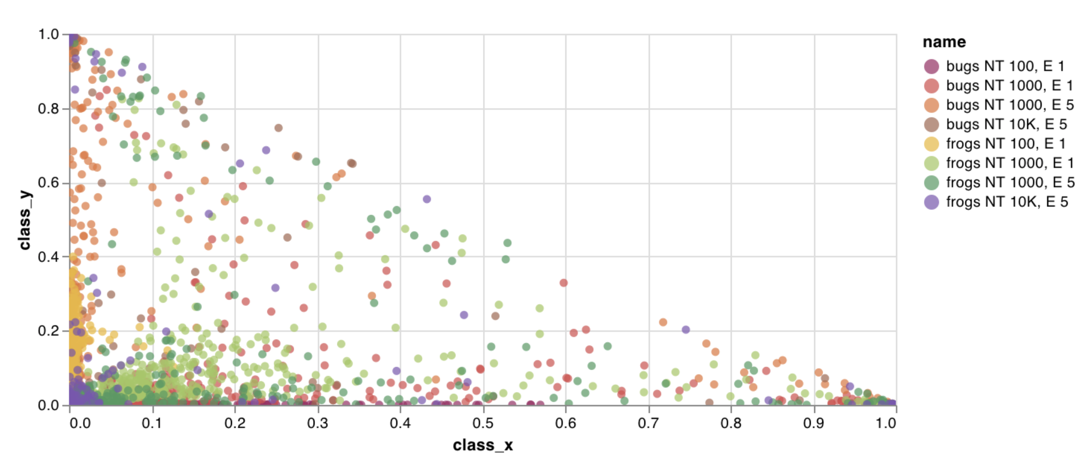
wandb.plot.scatter()
カスタム散布図 (任意の軸xとyのペア上のポイント (x、y) のリスト) を記録します。
data = [[x, y] for (x, y) in zip(class_x_scores, class_y_scores)]
table = wandb.Table(data=data, columns=["class_x", "class_y"])
wandb.log({"my_custom_id": wandb.plot.scatter(table, "class_x", "class_y")})
これを使用して、任意の2つの次元で散布ポイントを記録できます。2つの値のリストを互いにプロットする場合、リスト内の値の数は正確に一致する必要があります。たとえば、各ポイントにはxとyが必要です。
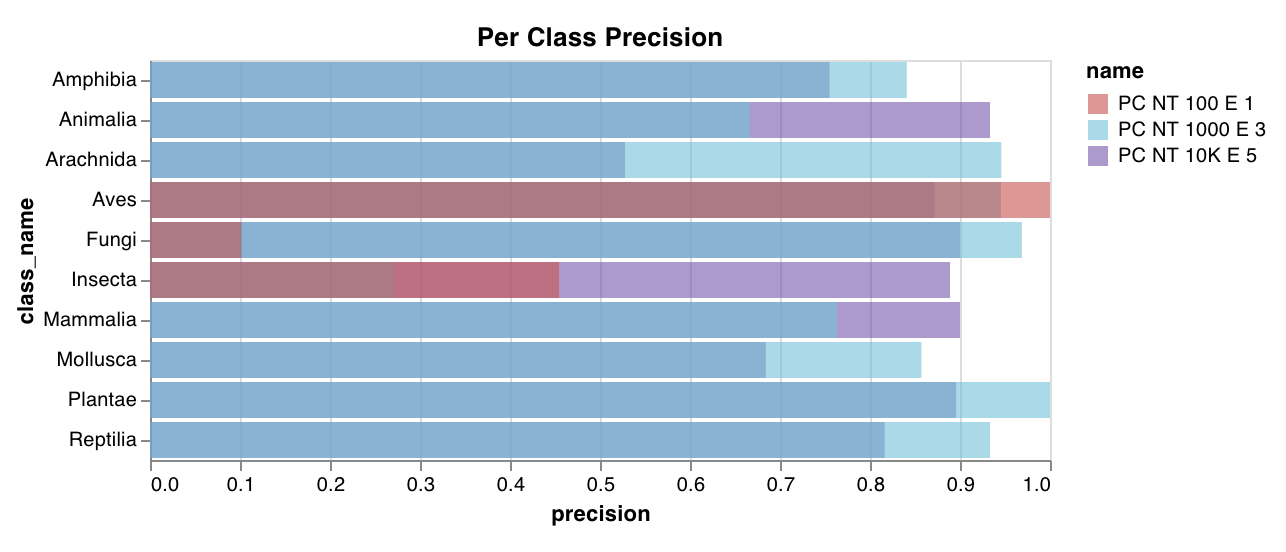
wandb.plot.bar()
カスタム棒グラフ (ラベル付きの値のリストを棒として表示) を数行でネイティブに記録します。
data = [[label, val] for (label, val) in zip(labels, values)]
table = wandb.Table(data=data, columns=["label", "value"])
wandb.log(
    {
        "my_bar_chart_id": wandb.plot.bar(
            table, "label", "value", title="Custom Bar Chart"
        )
    }
)
これを使用して、任意の棒グラフを記録できます。リスト内のラベルと値の数は正確に一致する必要があります。各データポイントには、ラベルと値の両方が必要です。
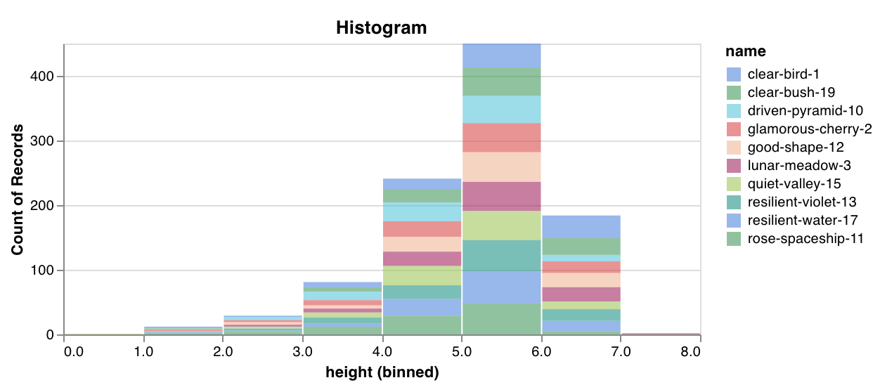
wandb.plot.histogram()
カスタムヒストグラム (値のリストを、出現のカウント/頻度でビンにソート) を数行でネイティブに記録します。予測信頼度スコアのリスト (scores) があり、その分布を可視化するとします。
data = [[s] for s in scores]
table = wandb.Table(data=data, columns=["scores"])
wandb.log({"my_histogram": wandb.plot.histogram(table, "scores", title="Histogram")})
これを使用して、任意のヒストグラムを記録できます。data は、行と列の2D配列をサポートすることを目的としたリストのリストであることに注意してください。
wandb.plot.line_series()
複数の線、または複数の異なるx-y座標ペアのリストを、1つの共有x-y軸セットにプロットします。
wandb.log(
    {
        "my_custom_id": wandb.plot.line_series(
            xs=[0, 1, 2, 3, 4],
            ys=[[10, 20, 30, 40, 50], [0.5, 11, 72, 3, 41]],
            keys=["metric Y", "metric Z"],
            title="Two Random Metrics",
            xname="x units",
        )
    }
)
xポイントとyポイントの数が正確に一致する必要があることに注意してください。複数のy値のリストに一致するx値のリストを1つ、またはy値のリストごとに個別のx値のリストを提供できます。
モデル評価グラフ
これらのプリセットグラフには、wandb.plot メソッドが組み込まれており、スクリプトから直接グラフをすばやく簡単に記録し、UIで探している正確な情報を確認できます。
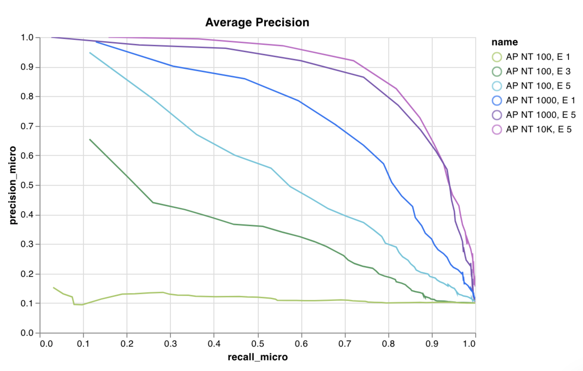
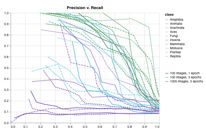
wandb.plot.pr_curve()
1行で PR曲線 を作成します。
wandb.log({"pr": wandb.plot.pr_curve(ground_truth, predictions)})
コードが以下にアクセスできる場合は、いつでもこれを記録できます。
- 例のセットに対するモデルの予測スコア (
predictions) - それらの例に対応する正解ラベル (
ground_truth) - (オプション) ラベル/クラス名のリスト (
labels=["cat", "dog", "bird"...]ラベルインデックス0がcat、1 = dog、2 = birdなどを意味する場合) - (オプション) プロットで可視化するラベルのサブセット (引き続きリスト形式)
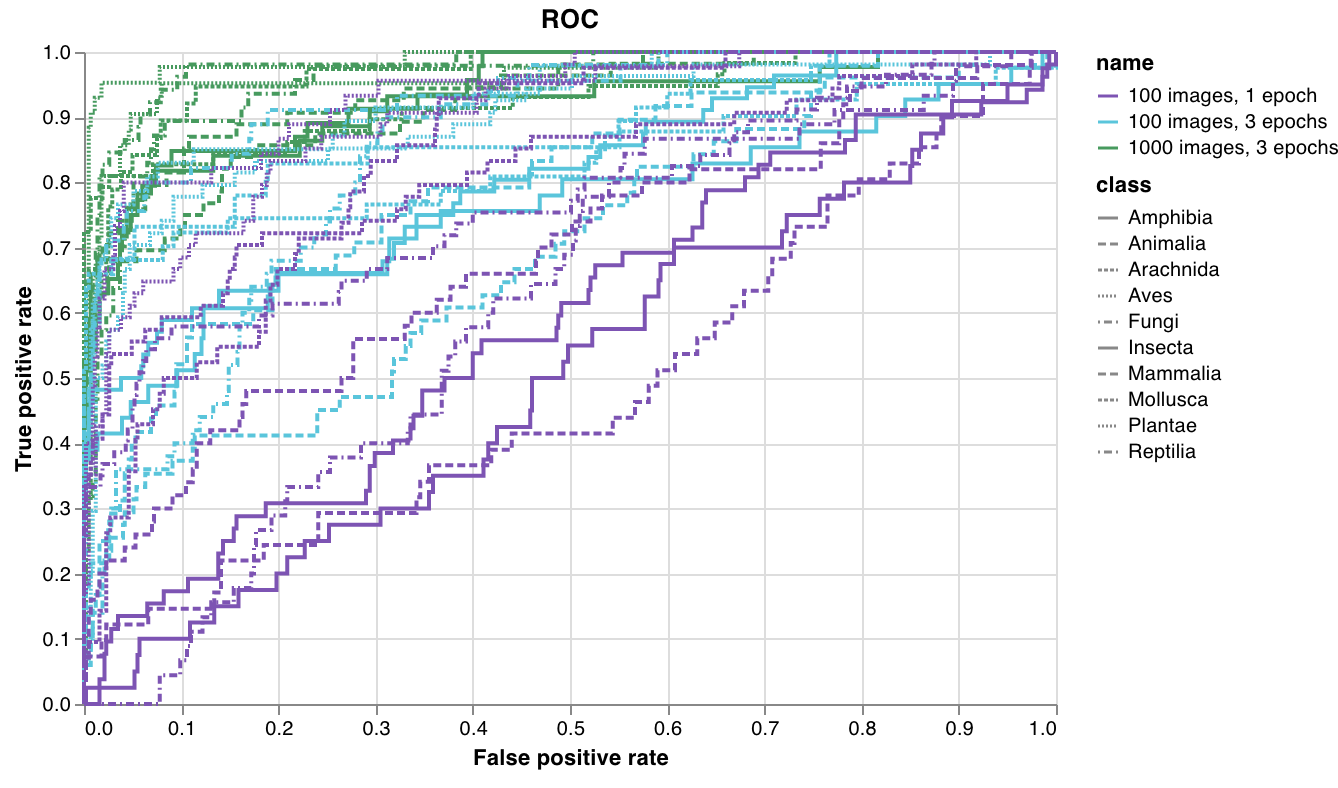
wandb.plot.roc_curve()
1行で ROC曲線 を作成します。
wandb.log({"roc": wandb.plot.roc_curve(ground_truth, predictions)})
コードが以下にアクセスできる場合は、いつでもこれを記録できます。
- 例のセットに対するモデルの予測スコア (
predictions) - それらの例に対応する正解ラベル (
ground_truth) - (オプション) ラベル/クラス名のリスト (
labels=["cat", "dog", "bird"...]ラベルインデックス0がcat、1 = dog、2 = birdなどを意味する場合) - (オプション) プロットで可視化するこれらのラベルのサブセット (引き続きリスト形式)
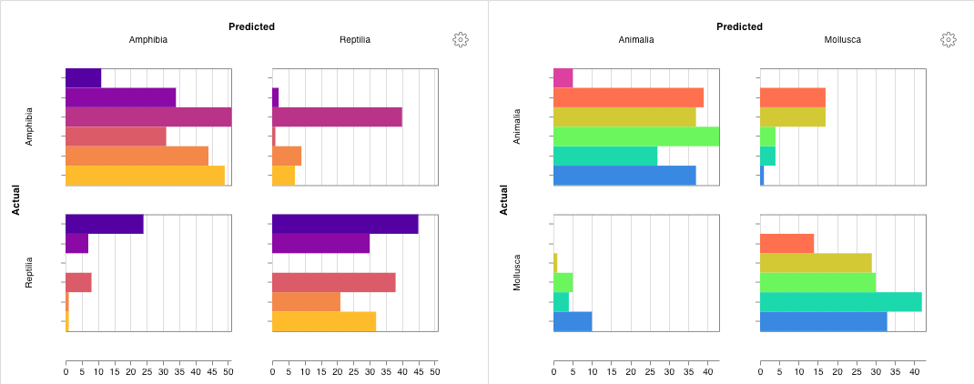
wandb.plot.confusion_matrix()
1行で多クラス 混同行列 を作成します。
cm = wandb.plot.confusion_matrix(
    y_true=ground_truth, preds=predictions, class_names=class_names
)

wandb.log({"conf_mat": cm})
コードが以下にアクセスできる場合は、いつでもこれを記録できます。
- 例のセットに対するモデルの予測ラベル (
preds) または正規化された確率スコア (probs)。確率は、(例の数、クラスの数) の形状である必要があります。確率または予測のいずれかを提供できますが、両方はできません。 - それらの例に対応する正解ラベル (
y_true) class_namesの文字列としてのラベル/クラス名の完全なリスト。例: インデックス0がcat、1がdog、2がbirdの場合、class_names=["cat", "dog", "bird"]。
アプリで表示
インタラクティブなカスタムグラフ
完全にカスタマイズするには、組み込みの カスタムグラフプリセット を調整するか、新しいプリセットを作成し、グラフを保存します。グラフIDを使用して、スクリプトからそのカスタムプリセットに直接データを記録します。
# プロットする列を含むテーブルを作成します
table = wandb.Table(data=data, columns=["step", "height"])

# テーブルの列からグラフのフィールドへのマッピング
fields = {"x": "step", "value": "height"}

# テーブルを使用して、新しいカスタムグラフプリセットを設定します
# 独自の保存されたグラフプリセットを使用するには、vega_spec_nameを変更します
# タイトルを編集するには、string_fieldsを変更します
my_custom_chart = wandb.plot_table(
    vega_spec_name="carey/new_chart",
    data_table=table,
    fields=fields,
    string_fields={"title": "Height Histogram"},
)
Matplotlib および Plotly プロット
wandb.plot を使用した W&B カスタムグラフ を使用する代わりに、matplotlib および Plotly で生成されたグラフを記録できます。
import matplotlib.pyplot as plt

plt.plot([1, 2, 3, 4])
plt.ylabel("some interesting numbers")
wandb.log({"chart": plt})
matplotlib プロットまたは figure オブジェクトを wandb.log() に渡すだけです。デフォルトでは、プロットを Plotly プロットに変換します。プロットを画像として記録する場合は、プロットを wandb.Image に渡すことができます。Plotly グラフも直接受け入れます。
fig = plt.figure() を使用してプロットとは別に figure を保存し、wandb.log の呼び出しで fig を記録できます。カスタム HTML を W&B Tables に記録する
W&B は、Plotly および Bokeh からのインタラクティブなグラフを HTML として記録し、それらを Tables に追加することをサポートしています。
Plotly figure を HTML として Tables に記録する
インタラクティブな Plotly グラフを HTML に変換して、wandb Tables に記録できます。
import wandb
import plotly.express as px

# 新しい run を初期化します
run = wandb.init(project="log-plotly-fig-tables", name="plotly_html")

# テーブルを作成します
table = wandb.Table(columns=["plotly_figure"])

# Plotly figure のパスを作成します
path_to_plotly_html = "./plotly_figure.html"

# Plotly figure の例
fig = px.scatter(x=[0, 1, 2, 3, 4], y=[0, 1, 4, 9, 16])

# Plotly figure を HTML に書き込みます
# auto_play を False に設定すると、アニメーション化された Plotly グラフが
# テーブル内で自動的に再生されるのを防ぎます
fig.write_html(path_to_plotly_html, auto_play=False)

# Plotly figure を HTML ファイルとして Table に追加します
table.add_data(wandb.Html(path_to_plotly_html))

# Table を記録します
run.log({"test_table": table})
wandb.finish()
Bokeh figure を HTML として Tables に記録する
インタラクティブな Bokeh グラフを HTML に変換して、wandb Tables に記録できます。
from scipy.signal import spectrogram
import holoviews as hv
import panel as pn
from scipy.io import wavfile
import numpy as np
from bokeh.resources import INLINE

hv.extension("bokeh", logo=False)
import wandb


def save_audio_with_bokeh_plot_to_html(audio_path, html_file_name):
    sr, wav_data = wavfile.read(audio_path)
    duration = len(wav_data) / sr
    f, t, sxx = spectrogram(wav_data, sr)
    spec_gram = hv.Image((t, f, np.log10(sxx)), ["Time (s)", "Frequency (hz)"]).opts(
        width=500, height=150, labelled=[]
    )
    audio = pn.pane.Audio(wav_data, sample_rate=sr, name="Audio", throttle=500)
    slider = pn.widgets.FloatSlider(end=duration, visible=False)
    line = hv.VLine(0).opts(color="white")
    slider.jslink(audio, value="time", bidirectional=True)
    slider.jslink(line, value="glyph.location")
    combined = pn.Row(audio, spec_gram * line, slider).save(html_file_name)


html_file_name = "audio_with_plot.html"
audio_path = "hello.wav"
save_audio_with_bokeh_plot_to_html(audio_path, html_file_name)

wandb_html = wandb.Html(html_file_name)
run = wandb.init(project="audio_test")
my_table = wandb.Table(columns=["audio_with_plot"], data=[[wandb_html], [wandb_html]])
run.log({"audio_table": my_table})
run.finish()
[i18n] feedback_title
[i18n] feedback_question
Glad to hear it! Please tell us how we can improve.
Sorry to hear that. Please tell us how we can improve.